CSE471_assignment
CSE471 Assignment | Blog
Paths to Equilibrium in Games | NeurIPS 2024
Original Authors: Bora Yongacoglu, Gürdal Arslan, Lacra Pavel, Serdar Yüisel
Blog Authors: Ashrafur Rahman, Fatema Tuj Johora, Mashroor Hasan Bhuiyan
Introduction
In this blog we break down the paper Paths to Equilibrium in Games presented at NeurIPS 2024. The paper deals with paths to equilibrium in finite normal-form games, a central topic in game-theory. In a finite normal-form game, there are \(n\) players who interact with each other and update their strategies to win. A very familiar example of such a game, is the game of Rock-Paper-Scissors.
The concept of winning or losing is generalised by defining rewards. Rewards are dictated by the combination of chosen strategies. The more reward a player gets, the better their strategy is. The goal of each player is to maximize their reward. Eventually, the game reaches a point where no player can improve their reward by changing their strategy. This is called a Nash Equilibrium.
Many different algorithms have been developed to find Nash Equilibrium in normal-form games. Particularly Multi-Agent Reinforcement Learning (MARL) algorithms have been used to find Nash Equilibrium in games. In Multi-Agent Reinforcement Learning, multiple agents interact within an environment and use the Reinforcement Learning technique to learn the best strategy to achieve their goals. In many of these algorithms, to limit the space of strategies, the agents are restricted to a constraint: if it is already responding best to the other agents’ strategies, it should not change its strategy. This is called the satisficing condition.
A sequence of strategies meeting the satisficing condition is called a satisficing path. Since, many MARL algorithms use satisficing paths to reach equilibrium, it is important to know if such paths always exist. So the key question is:
For a given game and starting strategy, can we always create a satisficing path that eventually leads to an equilibrium?
This paper focuses on answering this question and shows that for any finite \(n\)-player normal-form game and any starting strategy, it is always possible to create such a path. The study also shows that sometimes making counterintuitive changes to strategy changes, e.g. temporarily switching to strategies that lower rewards, are essential for reaching equilibrium.
Definitions:
Before we dive into the details of the paper, let’s define some key terms that will be used throughout the blog. We now define this terms informally. For the mathematically inclined, we will provide the formal definitions later.
Normal-Form Games
A normal-form game is a mathematical representation of a strategic interaction where a finite set of players each select a strategy simultaneously from their respective sets of available actions. The outcome of the game is determined by the combination of chosen strategies, with each player receiving a reward based on this outcome.
In other words, a normal-form game can be thought of as a table or a matrix where each row represents the action for one player and each column represents the action for another player. The cell or value at the intersection of a row and a column represents the reward or payoff for the corresponding players.
For example for a two-player game of rock-paper-scissors, the table would look like this:
| Rock | Paper | Scissors | |
|---|---|---|---|
| Rock | 0,0 | -1,1 | 1,-1 |
| Paper | 1,-1 | 0,0 | -1,1 |
| Scissors | -1,1 | 1,-1 | 0,0 |
In this table, the rows represent the actions of Player 1 (Rock, Paper, Scissors) and the columns represent the actions of Player 2. The values in each cell represent the rewards for Player 1 and Player 2 respectively. For example, if Player 1 chooses Rock and Player 2 chooses Paper, Player 1 loses 1 and Player 2 wins 1. So, Player 1 receives a reward of -1 and Player 2 receives a reward of 1.
Notice that in this game, there is no state or history involved. The players make their decisions simultaneously and independently. And the rewards are determined by the combination of actions chosen by the players.
Strategies
Strategies are the choices made by players in a game. For the game above a possible strategy for Player 1 could be to always choose Rock. Player 2 could always choose Paper.
These are pure strategies. Strategies where a player chooses a single action with probability 1.
In a normal-form game, players can also use mixed strategies where they choose actions with certain probabilities. For example if Player 1 chooses Rock with probability 0.5 and Paper with probability 0.5, this is a mixed strategy.
In this blog, when we refer to strategies, we are referring to mixed strategies unless otherwise specified.
Strategy Profile
A strategy profile is a collection of strategies, one for each player in the game.
For example, in the rock-paper-scissors game, if Player 1 chooses Rock with probability 0.5 and Paper with probability 0.5, and Player 2 chooses Paper with probability 0.5 and Scissors with probability 0.5. Then the strategy profile would be (Rock: 0.5, Paper: 0.5) for Player 1 and (Paper: 0.5, Scissors: 0.5) for Player 2.
Best Responding Strategy
Best Responding Strategy is the strategy that maximizes a player’s payoff, given the strategies chosen by other players. It is a rational choice based on the idea that other players’ strategies stay the same, so the player cannot improve their payoff by changing their own strategy.
For example, if Player 2 always chooses Paper, then the best responding strategy for Player 1 would be to always choose Scissors.
Satisfied Players
Satisfied Players are those who are already using a best responding strategy to their opponents’ current strategies. These players are already getting optimal reward considering the present strategies of other players. Therefore, it is intuitive to keep their strategies unchanged.
Unsatisfied Players
Unsatisfied Players are not using the best responding strategy but they can improve their reward by changing their strategy. These players are in a suboptimal situation and can increase their payoff by changing their strategy.
Nash Equilibrium
A Nash equilibrium is a concept in game theory that describes a set of strategies or a strategy profile, such that no player has an incentive to unilaterally change their strategy. In other words, a Nash equilibrium is a set of strategies where each player’s strategy is optimal given the strategies of the other players. So, we can say that a Nash equilibrium is a state of the game where all players are satisfied.
In the Rock-Paper-Scissors game, a Nash equilibrium would be if both players choose each action with probability 1/3. Because in this case, no player can improve their reward by changing their strategy.
Consider another example. Imagine a group of friends deciding what to do on a weekend. Each friend has their preferences (movies, bowling, or staying home), and their happiness depends not only on what they choose but also on what others decide. A Nash equilibrium happens when everyone has made their choice, and no one can be happier by changing their mind—as long as everyone else sticks to their own decision.
Multi-Agent Reinforcement Learning (MARL)
Multi-Agent Reinforcement Learning (MARL) is a subfield of reinforcement learning where multiple agents interact within an environment to achieve individual or collective goals. Each agent learns to make decisions by interacting with the environment and receiving feedback in the form of rewards.
MARL algorithms are often used to find Nash Equilibrium in games. These algorithms use a combination of reinforcement learning techniques and game theory concepts to help agents learn the best strategies to reach equilibrium.
Satisficing Paths
A satisficing path is a sequence of strategy profiles where satisfied players (those already using their best response) do not change their strategies, and unsatisfied players freely explore new strategies. The idea is that satisfied players are already in a good position, so they don’t need to change their strategies, while unsatisfied players can explore new strategies to improve their rewards. Many existing MARL algorithms use satisficing paths to reach equilibrium.
Problem Statement
The authors investigate whether satisficing paths can always lead to a Nash equilibrium in finite normal-form games.
Core Question
For any finite normal-form game and any initial strategy profile, can we construct a satisficing path that guarantees convergence to Nash equilibrium?
Results
The paper proves that such a path always exists. Interestingly, this result leverages suboptimal updates—a departure from conventional reward improving approaches to achieve equilibrium and avoid cyclical behaviors.
Mathematical Framework
Now that we have a basic understanding of what the paper is about, we make things a bit more concrete by introducing the mathematical framework used in the paper.
Game Representation
A finite \(n\)-player normal-form game \(\Gamma\) is defined by a tuple \((n, \mathbf{A}, \mathbf{r})\), where:
-
\(n\): Number of players.
We often denote the set of players as \([n] = \{1, 2, \ldots, n\}\).
-
\(\mathbf{A} = \mathbb{A}^1 \times \mathbb{A}^2 \times \cdots \times \mathbb{A}^n\): Set of joint actions.
Here each set \(\mathbb{A}^i\) represents the action set for player \(i\).
-
\(\mathbf{r} = (r^1, r^2, \ldots, r^n)\): Reward functions.
Here \(r^i: \mathbf{A} \to \mathbb{R}\) specifies the reward for player \(i\) for each joint action \(\mathbf{a} \in \mathbf{A}\).
Description of Play
Each player selects a mixed strategy \(x^i \in \mathcal{X}^i = \Delta_{\mathbb{A}^i}\), where \(\Delta_{\mathbb{A}^i}\) is the set of probability distributions over the action set \(\mathbb{A}^i\). That is, each player assigns some probability to each action in their action set.
The combination of mixed strategies chosen by all players is called the strategy profile \(\mathbf{x} = (x^1, x^2, \ldots, x^n) \in \mathbf{X} = \mathcal{X}^1 \times \mathcal{X}^2 \times \cdots \times \mathcal{X}^n\).
To denote the strategies of all players except \(i\), we use \(\mathbf{x}^{-i} = (x^1, x^2, \ldots, x^{i-1}, x^{i+1}, \ldots, x^n) \in \mathbf{X}^{-i}\).
Each player selects their mixed strategy independently and simultaneously without knowing the strategies chosen by other players. Each player then samples an action according to their mixed strategy, \(a^i \sim x^i\) and receives a reward \(r^i(\mathbf{a})\) based on the joint action \(\mathbf{a} = (a^1, a^2, \ldots, a^n)\).
Objective
Each player tries to maximize their expected reward, which is the expected value of their reward function given by the mixed strategies chosen by all players:
\[R^i(\mathbf{x}) = \mathbb{E}_{\mathbf{a} \sim \mathbf{x}}[r^i(\mathbf{a})]\]Best Response
A mixed strategy \(x^i_\star \in \mathcal{X}^i\) is a best response to the mixed strategies of other players \(\mathbf{x}^{-i} \in \mathbf{X}^{-i}\) if it maximizes the expected reward of player \(i\):
\[x_\star^i \in \text{BR}^i_0(\mathbf{x}^{-i}) \quad \text{if} \quad R^i(x_\star^i, \mathbf{x}^{-i}) \geq R^i(x^{i}, \mathbf{x}^{-i}) \quad \text{for all} \quad x^{i} \in X^i\]Here \(\text{BR}^i_0(\mathbf{x}^{-i})\) is the set of mixed strategies that are best responses to \(\mathbf{x}^{-i}\).
Satisficing Paths
A sequence of strategy profiles \((x_t)_{t\ge 1}\) is a satisficing path if, for every \(t \ge 1\), for all the players \(i \in [n]\): \(x^i_t \in \text{BR}^i_0(x_{t-1}^{-i}) \Rightarrow x^i_{t + 1} = x^i_t\)
Nash Equilibrium
A strategy profile \(\mathbf{x}_\star = (x_1^\star, x_2^\star, \ldots, x_n^\star)\) is a Nash equilibrium if no player can unilaterally improve their reward by changing their strategy. That is if,
\[x^i_\star \in \text{BR}^i_0(\mathbf{x}_\star^{-i}) \quad \text{for all} \quad i \in [n]\]Theorem 1
The central contribution of the paper is the following theorem:
Any finite normal-form game \(\Gamma\) has the satisficing paths property. That is, for any \(x_1 \in X\), there exists a satisficing path \((x_1 , x_2, \dots, x_T)\) such that, for some finite \(T=T(x_1)\), the strategy profile \(x_T\) is a Nash equilibrium.
The proof is very long and involves a lot of mathematical rigour. So, we defer the full proof to the end of the blog for those who are interested in the details. We outline the proof in a more informal way in the next section. The curious readers are encouraged to take the time to read the enitre proof for an excting journey.
Proof Outline
For a normal-form game \(\Gamma\), we construct a sequence of strategy profiles \((\mathbf{x}_t)_{t=1}^{T}\) that satisfies the conditions of a satisficing path, starting from an initial strategy profile \(\mathbf{x}_1\) and ending at a Nash equilibrium \(\mathbf{x}_T\).
- We iteratively construct \(\mathbf{x}_{t+1}\) from \(\mathbf{x}_{t}\) starting from \(\mathbf{x}_1\).
- Choose \(\mathbf{x}_{t+1}\) after \(\mathbf{x}_t\) such that:
- \(\mathbf{x}_{t+1}\) satisfies the satisficing path condition.
- \(\mathbf{x}_{t+1}\) increases the number of unsatisfied players.
- The process continues until we reach a strategy profile \(\mathbf{x}_T\) where no more unsatisfied players can be added.
-
At this point, we either have a strategy profile with all unsatisfied players or a mix of satisfied and unsatisfied players.
Case 1: If all players are unsatisfied, we can make any update to reach a Nash equilibrium \(\mathbf{x}_T\) in one step.
Case 2: If we have a mix of satisfied and unsatisfied players, we can still reach a Nash equilibrium \(\mathbf{x}_T\) at once by changing the strategies of only the unsatisfied players.
This construction iterative builds a satisficing path to a Nash equilibrium in at most \(n\) steps. This proves the theorem on a high level. The detailed proof is provided at the end of the blog.
Insights and Implications
Key Takeaways
-
Convergence Assurance: Satisficing paths guarantee convergence to Nash equilibrium in finite normal-form games. Thereore, algorithms that follow satisficing paths can be assured of reaching equilibrium.
-
Sub-optimal Updates: Always choosing the best response for each player often leads to cyclical behaviors in adversial dynamics, i.e. if the game is non-cooperative, the players may never reach equilibrium and cycle between strategies that benefit one player at the expense of others. Choosing sub-optimal updates can help in reaching equilibrium more effectively.
-
Distributed Applicability: This approach can be implemented in decentralized systems since each player can locally estimate if they are satisfied or unsatisfied. However, finding the best response may require global information which is not needed in this approach.
Implications for MARL
-
Exploration and Exploitation: The satisficing principle enables exploration with some degree of randomness when the players are unsatisfied. While it also allows exploitation by maintaining the current strategy when satisfied.
-
Alternating between Reward Improving and Suboptimal Periods: As the proof shows, sometimes making suboptimal changes to strategies is essential for reaching equilibrium. This insight can be used to design MARL algorithms that alternate between reward-improving and suboptimal periods to reach equilibrium more effectively.
Broader Applications
Markov Games:
A Markov game is the stateful generalization of a normal-form game. It extends the concept of normal-form games to multi-state and multi-player settings. In Markov games, players interact with each other and the environment in a sequential manner, where the state of the environment changes based on the actions taken by the players.
The results of this paper can be extended to Markov games, providing a theoretical foundation for MARL algorithms in more complex environments. Unfortunately, the proof technique used in the paper doesn’t readily extend to Markov games. However, that doesn’t suggest that the results are not applicable to Markov games but the necessity of different proof techniques.
Decentralized Learning
In many cases players can evaluate their strategy compared to an optimal strategy, even when they only have partial information. In decentralized algorithms, each player only has access to partial or local information. The satisficing principle can be applied in these scenarios to help agents reach equilibrium without requiring global information.
The “win–stay” part of the satisficing principle serves as a local stopping condition. Players can estimate if they are satisfied or unsatisfied based on their local information. If they are satisfied, they can stop updating their strategy. If not they aren’t required to know the global state of the game since they don’t need to find the best response.
Future Works
Future work could focus on:
- Extending results to multi-state Markov games and continuous-action spaces.
- Incorporating \(\epsilon\)-best responses to account for small estimation errors.
- Developing efficient algorithms to construct satisfying paths in large-scale and decentralized systems.
Proof of Theorem 1
Before starting the proof, we introduce some notations and functions and their properties that will be needed in the proof.
Some Notations
Let \(\Gamma\) be a finite \(n\)-player normal-form game.
Let \(\mathbf{x} \in \mathbf{X}\) be a mixed strategy profile at some time step.
Based on \(\mathbf{x}\), we can divide the players \([n]\) in to two disjoint sets,
-
Satisfied Players:
\[\text{Sat}(\mathbf{x}) = \{i \in [n] : x_i \in \text{BR}^i_0(x_{-i})\}\]The players whose strategies are a best response to their opponents’ strategies \(\mathbf{x}^{-i}\).
-
Unsatisfied Players:
\[\text{UnSat}(\mathbf{x}) = \{i \in [n] : x_i \notin \text{BR}^i_0(x_{-i})\} \\ = [n] \setminus \text{Sat}(x) \\\]The players whose strategies are not a best response to their opponents’ strategies.
Some subsets of the set strategies \(\mathbf{X}\) is of particular interest to us:
-
Acessible Strategies \(\text{Access}(\mathbf{x})\):
\[\text{Access}(\mathbf{x}) = \{ \mathbf{y} \in \mathbf{X}: y^i=x^i, \forall i \in \text{Sat}(\mathbf{x}) \}\]These are the strategies that can be chosen after \(\mathbf{x}\) since we are restricting the paths to be satisficing. The strategies that can be chosen after \(\mathbf{x}\) must share the same strategy for the players in \(\text{Sat}(\mathbf{x})\).
-
No Better Strategies \(\text{NoBetter}(\mathbf{x}) \subseteq \text{Access}(\mathbf{x})\):
\[\text{NoBetter}(\mathbf{x}) = \{ \mathbf{y} \in \text{Access}(\mathbf{x}): \text{UnSat}(\mathbf{x}) \subseteq \text{UnSat}(\mathbf{y}) \}\]These are the accessible strategies that do not satisfy any player who were previously unsatisfied but might make a previously satisfied player unsatisfied. As a consequence, \(|\text{UnSat}(\mathbf{x_{t+1}})|\ge|\text{UnSat}(\mathbf{x_{t}})|\).
It is obvious that \(\mathbf{x} \in \text{NoBetter}(\mathbf{x})\) since \(\text{UnSat}(\mathbf{x}) \subseteq \text{UnSat}(\mathbf{x})\).
-
Worse Strategies \(\text{Worse}(\mathbf{x}) \subseteq \text{NoBetter}(\mathbf{x})\):
\[\text{Worse}(\mathbf{x}) = \{ \mathbf{y} \in \text{NoBetter}(\mathbf{x}): \text{UnSat}(\mathbf{x}) \subsetneq \text{UnSat}(\mathbf{y}) \}\]These are the accessible strategies that make the situation worse by making at least one previously satisfied player, unsatisfied. Additionally, all previously unsatisfied players remain unsatisfied as before. This means, \(|\text{UnSat}(\mathbf{x_{t+1}})|\geq|\text{UnSat}(\mathbf{x_{t}})+1|\).
\(\text{Worse}(\mathbf{x})\) can be empty (e.g. if \(\text{UnSat}(\mathbf{x}=[n]\)).
Expected Reward Function
The Expected Reward function \(R^i\) for player \(i\) is their expected reward which can be defined as:
\[R_i(\mathbf{x}) = \mathbb{E}_{\mathbf{A} \sim \mathbf{x}}[r^i(\mathbf{A})]\]It can be expressed as a sum of products:
\[R^i(\mathbf{x}) = \mathbb{E}_{\mathbf{A} \sim \mathbf{x}}[r^i(\mathbf{A})] \\ = \sum_{\mathbf{\bar{a}} \in \mathbf{A}} r^i(\mathbf{\bar{a}}) \mathbb{P}_{\mathbf{A} \sim \mathbf{x}}(\mathbf{A}=\bar{\mathbf{A}}) \\ = \sum_{\mathbf{\bar{a}} \in \mathbf{A}} r^i(\bar{a}^1,\dots,\bar{a}^n) \prod_{j=1}^n x_j(\bar{a}^j)\]We are summing over all possible actions \(\mathbf{a} \in \mathbf{A}\) of all players weighted by the probabilities of those actions under the mixed strategy profile \(\mathbf{x}\).
Some properties of the expected reward function is of interest to us:
-
\(R^i\) is a multi-linear function.
That is it is a linear function with respect to each of it’s parameter, the mixed strategy \(x^i\) of player \(i\). This can be easily seen since
\[R^i(x^i, \mathbf{x}^{-i}) = \sum_{\mathbf{\bar{a}} \in \mathbf{A}} \left [ r^i(\bar{a}^1,\dots,\bar{a}^n) \prod_{j \neq i} x^j(\bar{a}^j) \right ] x^i(\bar{a}^i) \\ = \sum_{\mathbf{\bar{a}} \in \mathbf{A}} w_{\mathbf{x}^{-i}}(\mathbf{\bar{a}}) x^i(\bar{a}^i)\]Here, \(w_{\mathbf{x}^{-i}}(\mathbf{\bar{a}}) \in \mathbb{R}\) is constant for a fixed \(\mathbf{x}^{-i}\) and \(\mathbf{\bar{a}}\). This means \(R_i(x^i, \mathbf{x}^{-i})\) is a linear function of \(x^i\) if \(\mathbf{x}^{-i}\) is fixed. Therefore, it is a multi-linear function of \(\mathbf{x}\).
-
\(R^i\) is continuous.
This follows from the fact that it is a multi-linear function.
-
Pure strategies attain the maximum expected reward when opponent strategies are fixed.
Formally speaking, for any player \(i\) and any mixed strategy profile \(\mathbf{x}^{-i}\),
\[\max_{x^i \in \Delta_{\mathbb{A}^i}} R^i(x^i, \mathbf{x}^{-i}) = \max_{a^i \in \mathbb{A}^i} R^i(\delta_{a^i}, \mathbf{x}^{-i})\]This is because for fixed opponent strategies, the expected reward function is linear. Upon fixing \(\mathbf{x}^{-i}\) the domain of \(R_i(x^i, \mathbf{x}^{-i})\) is the set of all mixed strategies for player \(i\): \(\Delta_{\mathbb{A}^i}\).
\[\Delta_{\mathbb{A}^i} = \{x^i \in \mathbb{R}^{\mathbb{A}^i}: \sum_{a^i \in \mathbb{A}^i} x^i(a^i) = 1, x^i(a^i) \geq 0\}\]This is the probability simplex over the set of actions \(\mathbb{A}^i\). It is a convex set, a convex shape in \(|\mathbb{A}^i|\) dimensional space. Maximisng a linear function over a convex set is a linear programming problem and the maximum is attained at the vertices of the convex set. The vertices of the probability simplex are the pure strategies.
To visualise this, consider a 3D probability simplex for a player with 3 actions \(\mathbb{A}^i = \{1,2,3\} \). The probability simplex is situated on the plane \(x+y+z=1\), with each axis representing the probability of choosing one of the actions.
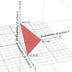
The maxima of a linear function over this triangle is attained at the vertices. Therefore, maxima are situated at either \((1,0,0)\), \((0,1,0)\) or \((0,0,1)\) which correspond to the pure strategies \(\delta_1\), \(\delta_2\) and \(\delta_3\) respectively.
Generalizing this to higher dimensions, the maximum value of the linear function \(R^i(x^i, \mathbf{x}^{-i})\) when \(\mathbf{x}^{-i}\) is fixed, is attained at the pure strategies \(\{\delta_a^i: a^i \in \mathbb{A}^i\}\). Also note that if multiple pure strategies attain the maximum value, then any mixture of these pure strategies also attains the maximum value.
Property 3 is crucial for our proof. It implies that the maximum expected reward for player \(i\) when the opponents’ strategies are fixed is that of the maximizing pure strategy.
It also implies that if \(x^i\) is a best response to \(\mathbf{x}^{-i}\), then \(x^i\) must be a pure strategy or a mixture of pure strategies which are best responses.
We state this formally as a lemma.
Lemma 1
\(x^i\) is a best response to \(\mathbf{x}^{-i}\) if and only if \(x^i\) is a mixture of pure strategies which are individually best responses to \(\mathbf{x}^{-i}\). Formally, \(x^i \in \text{BR}^i_0(\mathbf{x}^{-i})\) if and only if \(x^i(a^i) \gt 0 \Rightarrow \delta_{a^i} \in \text{BR}^i_0(\mathbf{x}^{-i})\).
In other words, if \(x^i\) is a best response to \(\mathbf{x}^{-i}\), then \(x^i\) must be supported on the set of maximizers \(\argmax_{a^i \in \mathbb{A}^i} \{ R^i(\delta_{a^i}, \mathbf{x}^{-i})\}\).
Auxillary Functions
We now discuss a set of functions we call the auxillary functions \(\{ F^i: i \in [n] \}\). They will come in handy later in the proof. The functions \(F^i: \mathbf{X} \to \mathbb{R}\) are defined as:
\[F^i(x^i, \mathbf{x}^{-i}) =\max_{a^i \in \mathbb{A}^i} R^i(\delta_{a^i}, \mathbf{x}^{-i}) - R^i(x^i, \mathbf{x}^{-i})\]We now discuss some properties of the auxillary functions, which are easy to justify thanks to the heavy lifting we did earlier.
For any \(i \in [n]\) and any strategy profile \((x^i, \mathbf{x}^{-i}) \in \mathbf{X}\) the following properties hold:
-
\(F^i\) is continuous.
This follows from the continuity of the expected reward function \(R^i\) as the pointwise maximum of finitely many continuous functions is continuous.
-
\(F^i \ge 0\) for all \(x \in \mathbf{X}\).
This follows from the definition of \(F^i\) and property 3 of the expected reward function. The maximum expected reward for player \(i\) when the opponents’ strategies are fixed is that of the maximizing pure strategy. Therefore, \(R^i(x^i, \mathbf{x}^{-i}) \le \max_{a^i \in \mathbb{A}^i} R^i(\delta_{a^i}, \mathbf{x}^{-i})\) for all \(x^i \in \Delta_{\mathbb{A}^i}\). This implies \(F^i(x^i, \mathbf{x}^{-i}) \ge 0\).
-
For any \(\mathbf{x}^{-1} \in \mathbf{X}^{-1}\), \(F^i(x^i, \mathbf{x}^{-i}) = 0\) if and only if \(i \in \text{Sat}(\mathbf{x})\), i.e. \(x^i \in \text{BR}^i_0(\mathbf{x}^{-i})\).
This again follows from the definition of \(F^i\) and property 3 of the expected reward function. \(F^i(x^i, \mathbf{x}^{-i}) = 0\) if and only if \(R^i(x^i, \mathbf{x}^{-i}) = \max_{a^i \in \mathbb{A}^i} R^i(\delta_{a^i}, \mathbf{x}^{-i}) = \max_{x^i \in \Delta_{\mathbb{A}^i}} R^i(x^i, \mathbf{x}^{-i})\), i.e. when the expected reward is maximum. This implies \(x^i\) is a best response to \(\mathbf{x}^{-i}\).
Proof
Okay, now that we are done with a quite a lot of preliminaries we can begin the actual proof.
Let \(\mathbf{x}_1 \in \mathbf{X}\) be any initial strategy. We now construct a satisficing path \(\mathbf{x}_1 , \mathbf{x}_2, \dots, \mathbf{x}_T\) of finite length \(T\) where \(\mathbf{x}_T\) is a Nash equilibrium.
Step 1: Check Initial Strategy
If \(\mathbf{x}_1\) is a Nash equilibrium we are done. Otherwise we continue to the next step.
Step 2: Iteratively Choose Worse Strategies
We iteratively produce a satisficing path \(\mathbf{x}_1 , \mathbf{x}_2, \dots, \mathbf{x}_t, \dots, \mathbf{x}_k\) as follows:
- We start with the initial strategy \(\mathbf{x}_1\) for \(t=1\).
- At each step, we arbitrarilly choose a worse strategy
so that the number of unsatisfied players increases.
We can choose \(\mathbf{x}_{t+1} \in \text{Worse}(\mathbf{x}_t)\) if \(\text{Worse}(\mathbf{x}_t) \neq \emptyset\). - If no worse strategy is accessible from \(\mathbf{x}_t\) at time step \(t\) we stop, i.e. if \(\text{Sat}(\mathbf{x}_t) = \emptyset\) (all players are already unsatisfied) or \(\text{Worse}(\mathbf{x}_t) = \emptyset\) (no worse strategy is accessible).
Step 3: Termination within at most \(n-1\) Steps
The above process terminates in at most \(n-1\) steps. Let \(i\) be the final step of the above process. We can show \(i \le n - 1\).
- Initially, \(|\text{UnSat}(\mathbf{x}_1)| \geq 1\) because \(\mathbf{x}_1\) is not a Nash equilibrium and so at least one player wasn’t satisfied.
- The number of unsatisfied players is strictly increasing at each time step.
- Even if at each step \(|\text{UnSat}(\mathbf{x}_t)|\) increases by 1, \(i\) can be at most \(n-1\).
Step 4: Check Final Strategy after Iteration
When \(\text{UnSat}(\mathbf{x}_k) = \emptyset\), the strategy profile \(\mathbf{x}_k\) satisfies the Nash equilibrium condition.
The process terminates at \(\mathbf{x}_k\) if either all players are unsatisfied or no worse strategy is accessible. Therefore, there are two cases:
Case 1: \(\text{Sat}(\mathbf{x}_k)=\emptyset\)
If all players are unsatisfied then the satisficing condition places no restrictions on the next strategy. Therefore, we can choose any strategy \(\mathbf{x}_{k+1} \in \mathbf{X}\), i.e. \(\text{Access}(\mathbf{x}_k) = \mathbf{X}\). We choose an arbitrary Nash equilibrium \(\mathbf{z}_\star\) and set \(\mathbf{x}_{k+1} = \mathbf{z}_\star\).
Therefore, taking \(T=k+1 \le n\) we have a satisficing path \(\mathbf{x}_1 , \mathbf{x}_2, \dots, \mathbf{x}_k, \mathbf{z}_\star\) where \(\mathbf{z}_\star\) is a Nash equilibrium. We are done.
Case 2: \(\text{Sat}(\mathbf{x}_k)\ne\emptyset\) and \(\text{Worse}(\mathbf{x}_k)=\emptyset\)
This is the trickier case. We need to show there exists a Nash equilibrium \(\mathbf{x}_\star\) such that \(\mathbf{x}_\star \in \text{Access}(\mathbf{x}_k)\).
Step 5: Find the Nash equilibrium \(\mathbf{x}_\star\)
Since \(\text{Sat}(\mathbf{x}_k)\ne\emptyset\), we cannot change the strategies of satisfied players \(\text{Sat}(\mathbf{x}_k)\). Let \(m = |\text{Sat}(\mathbf{x}_k)|\) be the number of satisfied players. We can only change the strategies of \(n-m\) unsatisfied players \(\text{UnSat}(\mathbf{x}_k)\).
We can create a new game \(\bar{\Gamma}\) with \(n-m\) players by restricting the strategy space of the satisfied players to their current strategies. Let \(\mathbf{\bar{x}}_\star\) be a Nash equilibrium of the new game \(\bar{\Gamma}\). We can extend \(\mathbf{\bar{x}}_\star\) to a Nash equilibrium \(\mathbf{x}_\star\) of the original game \(\Gamma\) by setting the strategies of the satisfied players to their strategies in \(\mathbf{x}_k\). That is we set,
\[x^i_\star = \begin{cases} x^i_k, &\text{ if } i \in \text{Sat}(\mathbf{x}_k), \\ \bar{x}^i_\star, &\text{ if } i \in \text{UnSat}(\mathbf{x}_k). \end{cases}\]Since \(x^i_k = x^i_{\star}\) for \(i \in \text{Sat}(\mathbf{x}_k)\), \(\mathbf{x}_\star \in \text{Access}(\mathbf{x}_k)\).
Therefore, we can set \(T=k+1 \le n\) and \(\mathbf{x}_T = \mathbf{x}_\star\) and we have a satisficing path \(\mathbf{x}_1 , \mathbf{x}_2, \dots, \mathbf{x}_k, \mathbf{x}_T\) where \(\mathbf{x}_T\) is a Nash equilibrium. And we are done with the construction of the satisficing path to a Nash equilibrium from any initial strategy \(\mathbf{x}_1 \in \mathbf{X}\).
But wait! We didn’t proof that \(\mathbf{x}_\star\) is indeed a Nash equilibrium. We need to show that \(\mathbf{x}_\star\) is a Nash equilibrium of the original game \(\Gamma\). So, here comes the hard part.
Proof: \(\mathbf{x}_\star\) is a Nash equilibrium of \(\Gamma\)
The way we constructed \(\mathbf{x}_\star\) from \(\mathbf{\bar{x}}_\star\), the players unsatisfied in \(\mathbf{x}_k\) are satisfied in \(\mathbf{x}_\star\).
This is because \(\mathbf{\bar{x}}_\star\) is a Nash equilibrium of the restricted game \(\bar{\Gamma}\) we considered where only the the unsatisfied players \(\text{UnSat}(\mathbf{x}_k)\) were allowed to change their strategies. In a Nash equilibrium all the players are satisfied. Therefore, the players \(\text{UnSat}(\mathbf{x}_k)\) must be satisfied in \(\mathbf{\bar{x}}_\star\).
\[\text{UnSat}(\mathbf{x}_k) \subseteq \text{Sat}(\mathbf{x}_\star)\]What remains to be shown is,
\[\text{Sat}(\mathbf{x}_k) \subseteq \text{Sat}(\mathbf{x}_\star)\]The satisfied players \(\text{Sat}(\mathbf{x}_k)\) should also satisfied in \(\mathbf{x}_\star\).
Here our old friends, the auxillary functions, come to the rescue. Using the auxillary functions, a bit of algebra and limits of sequences, we can show that the satisfied players \(\text{Sat}(\mathbf{x}_k)\) are also satisfied in \(\mathbf{x}_\star\).
But before that, a simple observation.
In the case we are dealing with,
\(\text{Sat}(\mathbf{x}) \ne \emptyset\) and \(\text{Worse}(\mathbf{x}_k)=\emptyset\). So, there is no worse
strategy in \(\text{NoBetter}(\mathbf{x}_k)\) which unsatisfy a previously satisfied player
\(i \in \text{Sat}(\mathbf{x}_k)\). This leads to the following:
Observation 1: For any strategy \(\mathbf{y} \in \text{NoBetter}(\mathbf{x}_k)\), the satisfied players in \(\mathbf{x}_k\) are also satisfied in \(\mathbf{y}\). That is, \( \text{Sat}(\mathbf{x}_k) \subseteq \text{Sat}(\mathbf{y})\)
Now if only we could show that \(\mathbf{x}_\star \in \text{NoBetter}(\mathbf{x}_k)\), we would be done.
But that is impossible because \(\text{UnSat}(\mathbf{x}_k) \subseteq \text{Sat}(\mathbf{x}_\star)\). \(\mathbf{x}_\star\) satisfies the unsatisfied players in \(\mathbf{x}_k\). So, \(\mathbf{x}_\star\) can not be in \(\text{NoBetter}(\mathbf{x}_k)\).
Fortunately, though we can proof that a sequence of \(\text{NoBetter}(\mathbf{x}_k)\) strategies converges to \(\mathbf{x}_\star\).
Lemma 2
If \(\text{Worse}(\mathbf{x}_k) = \emptyset\), then there exists a sequence of strategies \(\{\mathbf{y}_t\}_{t=1}^\infty\) such that \(\mathbf{y}_t \in \text{NoBetter}(\mathbf{x}_k)\) for all \(t\) and \(\lim_{t \to \infty} \mathbf{y}_t = \mathbf{x}_\star\).
Before, we delve into the proof of the lemma, we need to brief about the algebra of the space of strategies \(\mathbf{X}\).
As noted before, the strategies \(x^i \in \mathcal{X}^i = \Delta_{\mathbb{A}^i}\), which is the probability simplex in \(\mathbb{R}^{\mathbb{A}^i}\). That is to say, the strategies are vectors in \(|\mathbb{A}^i|\) dimensional space. Therefore, \(\mathcal{X}^i\) inherits the Euclidean metric. Distance and neighbourhoods in \(\mathcal{X}^i\) are defined in terms of the familiar Euclidean metric, \(|x^i - y^i| = \sqrt{\sum_{a^i \in \mathbb{A}^i} (x^i(a^i) - y^i(a^i))^2}\).
Similarly, the Euclidean metric applies to the mixed strategy profile space \(\mathbf{X}\). For \(\mathbf{x}, \mathbf{y} \in \mathbf{X}\), the distance between \(\mathbf{x}\) and \(\mathbf{y}\) can be defined as,
\[|\mathbf{x} - \mathbf{y}| = \sqrt{\sum_{i=1}^n |x^i - y^i|^2}\]For \(\zeta > 0\), the \(\zeta\)-neighbourhood of a strategy profile \(\mathbf{x} \in \mathbf{X}\) can be defined as,
\[N_\zeta(\mathbf{x}) = \{\mathbf{y} \in \mathbf{X}: |\mathbf{x} - \mathbf{y}| < \zeta\}\]Neighbourhoods can be thoughts of as balls in high-dimensional space. It is a generalization of open sets \((x - \zeta, x + \zeta)\) in \(\mathbb{R}\) to higher dimensions.
Proof:
Recall the definition of limit of a sequence. A sequence \(\{\mathbf{y}_t\}_{t=1}^\infty\) converges to \(\mathbf{x}_\star\) if for any \(\zeta > 0\), there exists a \(T\) such that for all \(t \ge T\), \(\mathbf{y}_t \in N_\zeta(\mathbf{x}_\star)\). That is, there are \(\mathbf{y}_t\) arbitrarily close to \(\mathbf{x}_\star\).
For such a sequence to exist in , we need to show that for any \(\zeta > 0\), there exists a \(\mathbf{y}_t \in \text{NoBetter}(\mathbf{x}_k)\) such that \(\mathbf{y}_t \in N_\zeta(\mathbf{x}_\star)\).
We assume the contrary, that no such sequence exists. Then there exists an \(\zeta > 0\) such that there is no \(\mathbf{y} \in \text{NoBetter}(\mathbf{x}_k)\) such that \(\mathbf{y} \in N_\zeta(\mathbf{x}_\star)\). Which means,
\[\text{NoBetter}(\mathbf{x}_k) \cap N_\zeta(\mathbf{x}_\star) = \emptyset\]That is, there isn’t any \(\text{NoBetter}(\mathbf{x}_k)\) strategy in the \(\zeta\)-neighbourhood of \(\mathbf{x}_\star\). We can prove a contradiction if we can show that there exists a strategy \(\mathbf{z} \in \text{NoBetter}(\mathbf{x}_k) \cap N_\zeta(\mathbf{x}_\star)\). We need to find a strategy \(\mathbf{z} \in \text{NoBetter}(\mathbf{x}_k)\) strategy near \(\mathbf{x}_\star\).
We start by looking for \(\text{NoBetter}(\mathbf{x}_k)\) strategies in the neighbourhood of \(\mathbf{x}_k\).
We define \(\mathbf{w}_\xi \in \mathbf{X}\) for \(\xi \in (0,1]\) as follows,
\[w^i_\xi = \begin{cases} (1-\xi)x^i_k + \xi \text{Uniform}(\mathbb{A}^i), &\text{ if } i \in \text{UnSat}(\mathbf{x}_k) \\ x^i_k, & \text{ else. } \end{cases}\]Where, \(\text{Uniform}(\mathbb{A}^i)\) is the uniform distribution over the action set \(\mathbb{A}^i\).
\[\text{Uniform}(\mathbb{A}^i)(a^i) = \frac{1}{|\mathbb{A}^i|}\]Note that for \(i \in \text{UnSat}(\mathbf{x}_k)\), \(w^i_\xi\) is a mixture of the current strategy \(x^i_k\) and the uniform distribution over the action set \(\mathbb{A}^i\). The mixture is weighted by \(1-\xi\) and \(\xi\) respectively to ensure that \(w^i_\xi\) remains a probability distribution.
\(\mathbf{w}_\xi\) isn’t just any random set of strategy profiles. It has some interesting properties:
-
\(\mathbf{w}_{\xi} \in \text{Access}(\mathbf{x}_k)\).
Since only the strategies of the unsatisfied players are changed in \(\mathbf{w}_\xi\).
-
For \(i \in \text{UnSat}(\mathbf{x}_k)\), \(w^i_\xi\) is fully mixed.
That is, it assigns non-zero probability \(w^i_\xi(a^i)\) to every action \(a^i \in \mathbb{A}^i\) when \(i \in \text{UnSat}(\mathbf{x}_k)\). This follows from the definition of \(\text{Uniform}(\mathbb{A}^i)\). As \(\xi > 0\), every action \(a^i \in \mathbb{A}^i\) is assigned a non-zero probability of at least \(\xi/|\mathbb{A}^i|\).
-
\(\mathbf{w}_\xi \in N_\epsilon(\mathbf{x}_k)\), for sufficiently small \(\xi > 0\).
This can be seen by choosing \(\xi < \epsilon/2n\).
\[|\mathbf{x}_k - \mathbf{w}_\xi| = \sqrt{\sum_{i=1}^n \left |x^i_k - w^i_\xi \right |^2} = \sqrt{\sum_{i \in \text{UnSat}(\mathbf{x}_k)} \left |x^i_k - w^i_\xi\right |^2} \\ = \sqrt{\sum_{i \in \text{UnSat}(\mathbf{x}_k)} \left |x^i_k - (1-\xi)x^i_k - \xi \text{Uniform}(\mathbb{A}^i) \right |^2} \\ = \xi \sqrt{\sum_{i \in \text{UnSat}(\mathbf{x}_k)} \left |x^i_k - \text{Uniform}(\mathbb{A}^i) \right |^2} \\ \le \xi \sqrt{\sum_{i \in \text{UnSat}(\mathbf{x}_k)} 2^2} \le 2\xi \sqrt{\sum_{i \in [n]} 1} \lt 2n\xi \lt \epsilon\]Note that the last line can be understood if we consider that every \(x \in \Delta_{\mathbb{A}^i}\) is a vector in the \(|\mathbb{A}^i|\) dimensional hyper-sphere of radius 1, since probabilities sum to 1. So, \(|x-y| \le 2\) for all \(x,y \in \Delta_{\mathbb{A}^i}.\)
This shows that for any \(\epsilon > 0\), there is always a \(\xi > 0\) such that \(\mathbf{w}_\xi \in N_\epsilon(\mathbf{x}_k)\).
-
\(\mathbf{w}_\xi \in \text{NoBetter}(\mathbf{x}_k)\), for sufficiently small \(\xi > 0\).
This can be shown by considering the auxillary functions \(F^i\). By property 1 of the auxillary functions, \(F^i\) is continuous.
The value of a continuous function doesn’t change abruptly. That is to say, if we are close enough to a point where the function is positive, we can find a neighbourhood around that point where the function remains positive. This is the idea behind the following argument.
Property 3 of the auxillary functions says that \(F^i(\mathbf{x}_k) = 0\) if and only if \(i \in \text{Sat}(\mathbf{x}_k)\). For unsatisfied players \(i \in \text{UnSat}(\mathbf{x}_k)\), \(F^i(\mathbf{x}_k) > 0\).
We can take,
\[\sigma = \min_{i \in \text{UnSat}(\mathbf{x}_k)} F^i(w^i_\xi, \mathbf{x}^{-i}_k) > 0\]From the continuity of the auxillary functions, for all \(i \in \text{UnSat}(\mathbf{x}_k)\), there exists \(e_i > 0\) such that,
\[\mathbf{x} \in N_{e_i}(\mathbf{w}_\xi) \Rightarrow \left | F^i(\mathbf{x}) - F^i(\mathbf{x}_k) \right | < \frac{\sigma}{2}\]That is, there is a neighbourhood around \(\mathbf{x}_k\) where the value of \(F^i(\mathbf{x})\) is less than \(\sigma/2\) away from \(F^i(\mathbf{x}_k)\). Since, \(F^i(\mathbf{x}_k) \ge \sigma\), \(F^i(\mathbf{x})\) has to be more than \(\frac{\sigma}{2}\).
\[\left | F^i(\mathbf{x}) \right | \ge \left | F^i(\mathbf{x}_k) \right | - \left | F^i(\mathbf{x}) - F^i(\mathbf{x}_k) \right | > \sigma - \frac{\sigma}{2} = \frac{\sigma}{2}\]Therefore, for all \(i \in \text{UnSat}(\mathbf{x}_k)\), there is some \(e_i > 0\) such that \(F^i(\mathbf{x})\) is positive in the \(e_1\)-neighbourhood of \(\mathbf{x}_k\). Again, by property 3 of the auxillary functions, this implies for all \(i \in \text{UnSat}(\mathbf{x}_k)\), \(i\) is also unsatisfied in the \(e_1\)-neighbourhood of \(\mathbf{x}_k\).
Now we can extend this to all unsatisfied players, \(i \in \text{UnSat}(\mathbf{x}_k)\), if we Let
\[\bar{e} = \min_{i \in \text{UnSat}(\mathbf{x}_k)} e_i\]Since, \(\bar{e}\)-neighbourhood is a subset of \(e_i\)-neighbourhoods, i.e. \(N_{\bar{e}}(\mathbf{x}_k) \subseteq N_{e_i}(\mathbf{x}_k)\) for all \(i \in \text{UnSat}(\mathbf{x}_k)\), all unsatisfied players \(\text{UnSat}(\mathbf{x}_k)\) remain unsatisfied in the \(\bar{e}\)-neighbourhood of \(\mathbf{x}_k\). Therefore, we have,
\[\text{UnSat}(\mathbf{x}_k) \subseteq \text{UnSat}(\mathbf{x}), \text{ for all } \mathbf{x} \in N_{\bar{e}}(\mathbf{x}_k)\]So, now we know there is a neighbourhood around \(\mathbf{x}_k\) where all the unsatisfied players remain unsatisfied. We also know that \(\mathbf{w}_\xi\) is in the neighbourhood of \(\mathbf{x}_k\) by property 3. So taking \(\xi < \bar{e}/2n\), we have \(\mathbf{w}_\xi \in N_{\bar{e}}(\mathbf{x}_k)\). As a result,
\[\text{UnSat}(\mathbf{x}_k) \subseteq \text{UnSat}(\mathbf{w}_\xi)\]Also, by property 1, \(\mathbf{w}_\xi \in \text{Access}(\mathbf{x}_k)\). That means, \(\mathbf{w}_\xi \in \text{NoBetter}(\mathbf{x}_k)\) for sufficiently small \(\xi > 0\).
Now that we now we have a set \(\mathbf{w}_\xi\) of strategies in the neighbourhood of \(\mathbf{x}_k\). We need to show that one of these strategies is in the neighbourhood of \(\mathbf{x}_\star\).
So, we define another set of strategies \(\mathbf{z}_\lambda \in \mathbf{X}\) for \(\lambda \in (0,1]\) as follows,
\[z^i_\lambda = \begin{cases} (1-\lambda)x^i_\star + \lambda w^i_\xi, &\text{ if } i \in \text{UnSat}(\mathbf{x}_k) \\ x^i_k, & \text{ else. } \end{cases}\]\(\mathbf{z}_\lambda\) has properties similar to \(\mathbf{w}_\xi\) except that it is centered around \(\mathbf{x}_\star\).
-
\(\mathbf{z}_\lambda \in \text{Access}(\mathbf{x}_\star)\).
Since again, only the strategies of the unsatisfied players are changed in \(\mathbf{z}_\lambda\).
-
For \(i \in \text{UnSat}(\mathbf{x}_k)\), \(z^i_\lambda\) is fully mixed.
This is because \(w^i_\xi\) is fully mixed and \(\lambda > 0\), so each action \(a^i \in \mathbb{A}^i\) is assigned a non-zero probability of at least \(\xi\lambda/|\mathbb{A}^i|\).
-
\(\mathbf{z}_\lambda \in N_{\zeta}(\mathbf{x}_\star)\), for sufficiently small \(\lambda > 0\).
We can choose \(\lambda < \zeta/2n\) with a similar reasoning. Therefore for any \(\zeta > 0\), there is always a \(\lambda > 0\) such that \(\mathbf{z}_\lambda \in N_\zeta(\mathbf{x}_\star)\).
-
\(\mathbf{z}_\lambda \notin \text{NoBetter}(\mathbf{x}_k)\), for all \(\lambda \le \bar{\lambda}\) for some \(\bar{\lambda} > 0\).
This follows from property 3 and the assumption that \(\text{NoBetter}(\mathbf{x}_k) \cap N_\zeta(\mathbf{x}_\star) = \emptyset\) which we want to contradict.
By property 3, setting \(\lambda \le \bar{\lambda} < \zeta/2n\), we have \(\mathbf{z}_\lambda \in N_\zeta(\mathbf{x}_\star)\). Now if \(\mathbf{z}_\lambda \in \text{NoBetter}(\mathbf{x}_k)\), we have,
\[\mathbf{z}_\lambda \in \text{NoBetter}(\mathbf{x}_k) \cap N_\zeta(\mathbf{x}_\star)\]Which contradicts the assumption that \(\text{NoBetter}(\mathbf{x}_k) \cap N_\zeta(\mathbf{x}_\star) = \emptyset\). So, \(\mathbf{z}_\lambda \notin \text{NoBetter}(\mathbf{x}_k)\) for all \(\lambda \le \bar{\lambda}\).
Now that we have the tools at our disposal, we derive the contradiction.
From property 1 and 3 of \(\mathbf{z}_\lambda\), we know that for \(\lambda \in (0, \bar{\lambda}]\), \(\mathbf{z}_\lambda \in \text{Access}(\mathbf{x}_\star)\) but \(\mathbf{z}_\lambda \notin \text{NoBetter}(\mathbf{x}_k)\). This implies at least one player is satisfied at \(\mathbf{z}_\lambda\) who was unsatisfied at \(\mathbf{x}_k\).
Therefore, for all \(\lambda \in (0, \bar{\lambda}]\) there is a player \(i \in \text{UnSat}(\mathbf{x}_k)\) such that \(i \in \text{Sat}(\mathbf{z}_\lambda)\). But note that there are infinitely many \(\lambda\), but only finitely many players \([n]\).
So, there must be a player \(i^{\dagger} \in \text{UnSat}(\mathbf{x}_k)\) who is satisfied in infinitely many \(\mathbf{z}_\lambda\). In other words,
\[i^{\dagger} \in \text{Sat}(\mathbf{z}_\lambda) \Leftrightarrow z^{i^{\dagger}}_\lambda \in \text{BR}^{i^{\dagger}}_{0}\left (\mathbf{z}^{-i^{\dagger}}_\lambda\right ), \text{ for infinitely many } \lambda \in (0, \bar{\lambda}]\]We take a \(\lambda \in (0, \bar{\lambda}]\) such that \(z^{i^{\dagger}}_\lambda\) a best response to \(\mathbf{z}^{-i^{\dagger}}_\lambda\). Recall by property 3, \(\mathbf{z}_\lambda\) is a fully mixed strategy as \(i^{\dagger} \in \text{UnSat}(\mathbf{x}_k)\), so \(z^{i^{\dagger}}_\lambda(a^{i^{\dagger}}) > 0\) for all \(a^{i^{\dagger}} \in \mathbb{A}^{i^{\dagger}}\). By lemma 1, we have that all the pure strategies \(\{\delta_{a^{i^{\dagger}}}: a^{i^{\dagger}} \in\mathbb{A}^{i^{\dagger}}\}\) are also best responses to \(\mathbf{z}^{-i^{\dagger}}_\lambda\). Which means,
\[R^{i^{\dagger}}\left (z^{i^{\dagger}}_\lambda, \mathbf{z}^{-i^{\dagger}}_\lambda\right ) = R^{i^{\dagger}}\left (\delta_{a^{i^{\dagger}}}, \mathbf{z}^{-i^{\dagger}}_\lambda\right ), \text{ for all } a^{i^{\dagger}} \in \mathbb{A}^{i^{\dagger}}\]So, for any \(a, a’ \in \mathbb{A}^{i^{\dagger}}\), we have,
\[R^{i^{\dagger}}\left (\delta_{a}, \mathbf{z}^{-i^{\dagger}}_\lambda\right ) = R^{i^{\dagger}}\left (\delta_{a'}, \mathbf{z}^{-i^{\dagger}}_\lambda\right ) \\ \Leftrightarrow R^{i^{\dagger}}\left (\delta_{a}, \mathbf{z}^{-i^{\dagger}}_\lambda\right ) - R^{i^{\dagger}}\left (\delta_{a'}, \mathbf{z}^{-i^{\dagger}}_\lambda\right ) = 0 \\ \Leftrightarrow \sum_{\mathbf{a}^{-i^{\dagger}}} r^{i^{\dagger}}\left (a,\mathbf{a}^{-i^{\dagger}} \right ) \prod_{j\ne i^{\dagger}} (1-\lambda)x^j_\star(a^j) + \lambda w^j_\xi(a^j) - \sum_{\mathbf{a}^{-i^{\dagger}}} r^{i^{\dagger}}\left (a',\mathbf{a}^{-i^{\dagger}}\right ) \prod_{j\ne i^{\dagger}} (1-\lambda)x^j_\star(a^j) + \lambda w^j_\xi(a^j) = 0 \\ \Leftrightarrow \sum_{\mathbf{a}^{-i^{\dagger}}} \left [ r^{i^{\dagger}}\left (a,\mathbf{a}^{-i^{\dagger}}\right ) - r^{i^{\dagger}}\left (a',\mathbf{a}^{-i^{\dagger}}\right ) \right ] \prod_{j\ne i^{\dagger}} (1-\lambda)x^j_\star(a^j) + \lambda w^j_\xi(a^j) = 0\quad\quad\quad (1)\]The left hand side of \((1)\) is a polynomial in \(\lambda\) of degree at most \(n-1\). By the fundamental theorem of algebra, a polynomial of degree \(n - 1\) has at most \(n - 1\) roots. But we showed above that there are infinitely many \(\lambda \in (0, \bar{\lambda}]\) such that the above equation holds. This can only happen if the polynomial is identically zero. That is, the coefficients of the polynomial are all zero.
Therefore, \((1)\) holds for all \(\lambda \in (0, 1]\), meaning for any \(\lambda \in (0, 1]\), \(z^{i^{\dagger}}_\lambda \in \text{BR}^{i^{\dagger}}_{0}\left (\mathbf{z}^{-i^{\dagger}}_\lambda\right )\) and \(i^{\dagger} \in \text{Sat}(\mathbf{z}_\lambda)\).
Taking \(\lambda = 1\), we get, \( \mathbf{z}_1 = \mathbf{w}_\xi\). So, \(i^{\dagger} \in \text{Sat}(\mathbf{w}_\xi)\). Recall for sufficiently small \(\xi > 0\), \(\mathbf{w}_\xi \in \text{NoBetter}(\mathbf{x}_k)\). Therefore, \(i^{\dagger} \in \text{UnSat}(\mathbf{w}_\xi)\) implies \(i^{\dagger} \in \text{UnSat}(\mathbf{w}_\xi)\). A contradiction.
Thus, we see that there exists a sequence of strategies \(\{\mathbf{y}_t\}_{t=1}^\infty\) in \(\text{NoBetter}(\mathbf{x}_k)\) such that \(\lim_{t \to \infty} \mathbf{y}_t = \mathbf{x}_\star\). \(\square\)
Now that we have shown that there exists a sequence of strategies \(\{\mathbf{y}_t\}_{t=1}^\infty\) in \(\text{NoBetter}(\mathbf{x}_k)\) which converges to \(\mathbf{x}_\star\), from observation 1, we know that the satisfied players in \(\mathbf{x}_k\) are also satisfied in \(\mathbf{y}_t\) for all \(t\). That is,
\[\text{Sat}(\mathbf{x}_k) \subseteq \text{Sat}(\mathbf{y}_t)\]So it seems, the limit of \(\{\mathbf{y}_t\}_{t=1}^\infty\) should also satisfy \(\text{Sat}(\mathbf{x}_k)\). To mathematically show this, we again resort to our friends the auxillary functions.
By property 3 of \(F^i\), for all \(i \in \text{Sat}(\mathbf{x}_k)\), \(F^i(\mathbf{x}_k) = 0\). This also applies to \(\{\mathbf{y}_t\}\) as \(\text{Sat}(\mathbf{x}_k) \subseteq \text{Sat}(\mathbf{y}_t)\). Therefore we have,
\[F^i(\mathbf{y}_t) = 0, \text{ for all } t \in \mathbb{N} \text{ and } i \in \text{Sat}(\mathbf{x}_k)\]Since auxillary functions are continuous (property 1), \(\lim_{t \to \infty} F^i(\mathbf{y}_t)\) exists and is equal to value of the function at the limit point. Hence,
\[0 = \lim_{t \to \infty} F^i(\mathbf{y}_t) = F^i\left (\lim_{t \to \infty} \mathbf{y}_t\right ) = F^i(\mathbf{x}_\star), \text{ for all } i \in \text{Sat}(\mathbf{x}_k)\]This implies that for all \(i \in \text{Sat}(\mathbf{x}_k)\), \(i\) is also satisfied in \(\mathbf{x}_\star\). That is, \( \text{Sat}(\mathbf{x}_k) \subseteq \text{Sat}(\mathbf{x}_\star) \) And since, \( \text{UnSat}(\mathbf{x}_k) \subseteq \text{Sat}(\mathbf{x}_\star) \) by construction of \(\mathbf{x}_\star\), we have that,
\[\text{Sat}(\mathbf{x}_k) \cup \text{UnSat}(\mathbf{x}_k) = [n] = \text{Sat}(\mathbf{x}_\star)\]Therefore, \(\mathbf{x}_\star\) is indeed a Nash equilibrium. This finally, finally concludes the proof. \(\blacksquare\)
Application to Markov Games
Markov game is a generalization of both normal form games (multiplayer, singleton state) and Markov Decision Process (single player, multi state). There are \(n\) players and discounted rewards, described by a list \(\mathcal{G} = (n, \mathcal{S}, \mathcal{A}, \mathcal{T}, \mathbf{r}, \gamma)\), where \(\mathcal{S}\) is a finite set of states, \(\mathcal{A} = \mathcal{A}^1 \times \cdots \times \mathcal{A}^n\) is a finite set of action profiles, and \(\mathbf{r} = (r^1, r^2, \ldots, r^n)\) is a collection of reward functions, where \(r^i: \mathcal{S} \times \mathcal{A} \to \mathbb{R}\) describes the reward to player \(i\).
A transition probability function \(\mathcal{T} \in \mathcal{P}(\mathcal{S} \mid \mathcal{S} \times \mathcal{A})\) governs the evolution of the state process, described below, and a discount factor \(\gamma \in (0,1)\) is used to aggregate rewards across time.
Markov games refine the Nash equilibrium concept into Markov perfect equilibrium, which is a key focus for MARL algorithms. The authors have attempted to generalize Theorem 1 for Markov games too by conducting the proofs parallely.
To begin, one can construct a satisficing path \(\{\pi_1, \pi_2, \dots, \pi_k\}\) by growing the set of unsatisfied players at each iteration until either \(\text{UnSat}(\pi_k) = \{1, 2, \dots, n\}\) or \(\text{Worse}(\pi_k) = \emptyset\). In the latter case, one can consider the subgame involving only the players in \(\text{UnSat}(\pi_k)\) and obtain a Markov perfect equilibrium \(\tilde{\pi}_{\star}\) for that subgame, which can then be extended to a policy profile \(\pi_{\star} \in \text{Acc}(\pi_k)\) by putting
\[\pi^i_{\star}= \begin{cases} \tilde{\pi}^i_{\star}, &\text{ if } i \in \text{UnSat}(\pi_k), \\ \pi^i_k, &\text{ if } i \in \text{Sat}(\pi_k). \end{cases}\]Showing that this policy \(\pi_{\star} \in \Pi\) is a Markov perfect equilibrium of the \(n\)-player Markov game, extends Theorem 1 to Markov games. We can define \(\{f^i\}_{i = 1}^n\) analogous to the auxillary function \(\{F^i\}_{i = 1}^n\) defined for normal form games which satisfy same properties e.g. the continuity and semi-definiteness properties. Hence, one possible technique for completing this proof requires extending Lemma 2 to the multi-state case.
Unfortunately, the extension of Lemma 2 introduces unresolved states which breaks the analysis, and hence remains unproven.
Conclusion
The paper gives a theoretical foundation for the convergence of MARL algorithms to Nash equilibrium in normal-form games. The paper proofs satisficing paths can converge to Nash equilibrium. The proof construction gives insights for algorithm design and analysis in MARL. It shows that sometimes worse as opposed to best responding strategies can lead to convergence.
The theoretical guarantee provided by the paper can be used to improve MARL algorithms. It also explores the possibility of extending the results to Markov games and other more complex settings.
Endnotes
The paper is centered around the proof of one theorem, but it was a long and complex proof. We thought just presenting the outline of the proof and skipping all the mathematical details wouldn’t do justice to the elegance of the proof. So, we decided to to break it down in a way that is accessible to a wider audience. We hope that this blog was a first (hopefully satisfying) journey into mathematical rigour for some of the readers.
We hope you found it interesting. If there are any errors or suggestions, create an issue or pull request in the GitHub repository. Thank you for sticking to the end.